A simple model of moral hazard with limited liability

No monitoring case

import numpy as np
import matplotlib.pyplot as plt
from ipywidgets import interact
%matplotlib inline

Model Parameters

X = 200       #Project returns under success (=0 under failure)
p = 0.7       #probability of success if diligent
q = 0.5       #probability of success if non-diligent
I = 100
gamma = 1     # outside lenders' cost of funds
B = 20

F = 0        # Fixed cost of loan

Amax = 120

Amin = p*B/(p-q) -(p*X - gamma*I) + F

print('Expected project return {}'.format(p*X))
print('Expected cost of funds {}'.format(gamma*I+F))
print('LL rent at A=0 is {:5.1f}'.format(p*B/(p-q)))
print('Min collateral requirement is {:5.1f}'.format(Amin))
print('LL rent at A= Amin is {}'.format(-Amin+p*B/(p-q)))

Expected project return 140.0
Expected cost of funds 100
LL rent at A=0 is  70.0
Min collateral requirement is  30.0
LL rent at A= Amin is 40.0

** Intermediary fixed cost per borrower ** Set to zero in base case.

Monitoring technology: For simplicity and to fix ideas we assume a linear relationship betweeen more monitoring expense and the extent of moral hazard (the private benefits the client stands to capture from non-diligence)

B0 = 30
alpha = 0.4
def B(m): # Private benefit to non-diligence under monitoring intensity m
    return B0 - alpha*4

def B(m, B0=30, alpha=0.4):
    '''Private benefits as a function of monitoring m'''
    return B0 - alpha*m

Minimum collateral requirements

Bank Participation constraint:

\[p(X - s) + (1 - p)A \ge \gamma I + F\]

Incentive compatibility constraint when entrepreneur has pledgeable assets \(A\):

\[s \ge - A + \frac{B}{\Delta }\]

The limited liability constraint is written:

\[s \ge - A\]

Actually, a limited liability constraint must hold for each outcome state to make sure that the value of promised repayment in that state does not exceed the value of output plus any pledgeable collateral \(A\). In this two-state world the constraints are \((X - s) \le A\) and \((0 - s) \le A\), but the latter always binds first, so we focus only on this, re-written as stated above.

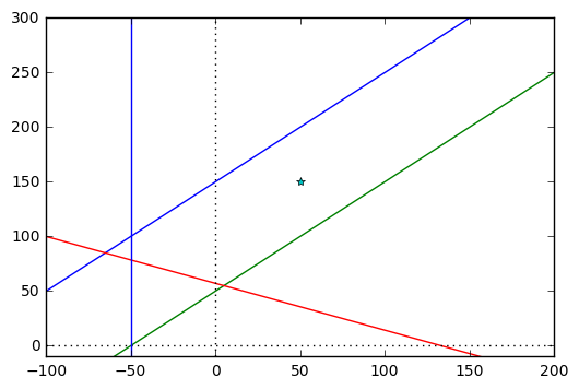
Diagram plots We want to plot the linear constraints and/or objectives lines in \(s_f - s_s\) space. For example a zero profit condition:

\[p(X-s_s)+(1-p)(0-s_f) - \gamma I - FC(N) = 0\]

can be rearanged to plot \(s_s\) as a function of \(s_f\):

\[s_s = X - \frac{\gamma I + F(N)}{p} -\frac{1-p}{p} s_f\]

Since we’ll be illustrating things below with a variety of plots, let’s try to economize on code by writing a simple ‘function factory’ call line_function(a,b) that allows to easily create multiple named and parameterized line functions and another plot_contraints() function that will plot a variable number of such lines.

def line_function(a, b):
    '''return a line function of the form f(x) = a + b*x'''
    def f(x):
        return a + b*x
    return f

def plot_constraints(*args, cfmin = -100, cfmax = 200):
    '''plot contract constraints
    Accepts a variable number of lines/constraint functions to plot
    on the same diagram'''
    cf = np.linspace(cfmin, cfmax, cfmax-cfmin+1)  # plot range
    for count, fn in enumerate(args):
        plt.plot(cf, fn(cf))
    plt.axhline(0, linestyle=':', color='black')
    plt.axvline(0, linestyle=':', color='black')
    plt.ylim(-10,300)

zeroprofit = line_function(X - I/p - F/p, -(1-p)/p)
ic0 = line_function(-0 + B(0)/(p-q), 1)
ic100 = line_function(-100 + B(0)/(p-q), 1)

plot_constraints(ic0, ic100, zeroprofit)
plt.plot(50,150, marker='*')
plt.axvline(-50)

<matplotlib.lines.Line2D at 0x7e45b70>